1D Search Methods

• In this section, we are interested in the problem of minimizing an objective function $f:\mathbb{R}\to\mathbb{R}$ (i.e., a one-dimensionla problem). The approach is to use an iterative search algorithm, also called a line-search method.
• In an iterative algorithm, we start with an initial candidate solution $x^{(0)}$ and generate a sequence of iterates $x^{(1)}, x^{(2)}, \cdots$. For eah iteration $k=0,1,2,\cdots,$ the next point $x^{(k+1)}$ depends on $x^{(k)}$ and the objective function $f$.
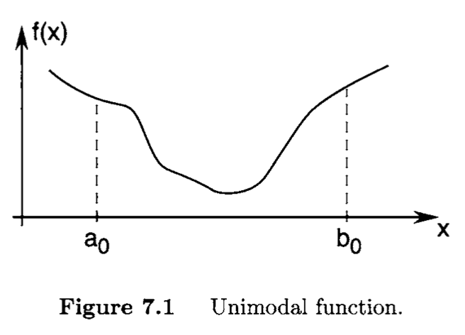
• The only property that we assume of the objective function $f$ is that it is unimodal, which means that $f$ has only one local minimizer.
• Our goal is to narrow the range prograssively until the minimizer is "boxed in" with sufficient accuracy.

Golden Section Search

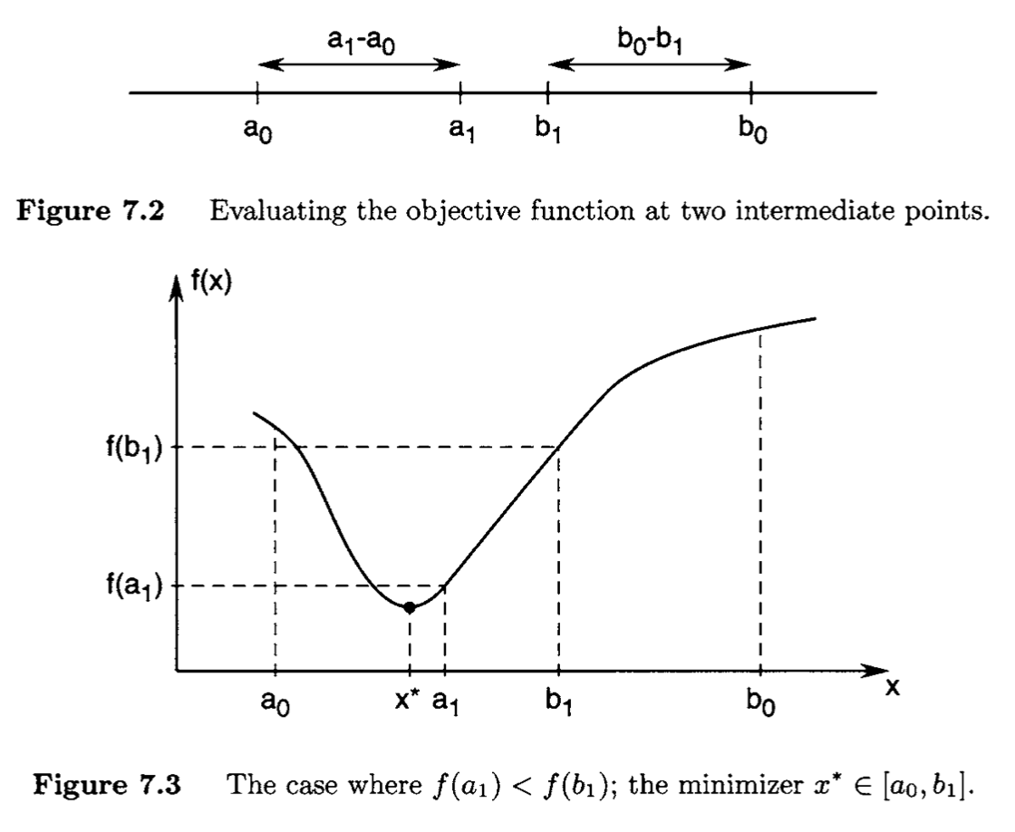
Consider a unimodel function $f$ of one variable and the interval $[a_0,b_0]$. Illustrated in Figure 7.2, we choose the intermediate points in such a way that the reduction in the range is symmetric, in the sense that

$$\begin{gather*} a_1-a_0=b_0-b_1=\rho(b_0,a_0), \rho<{1\over 2}. \end{gather*}$$

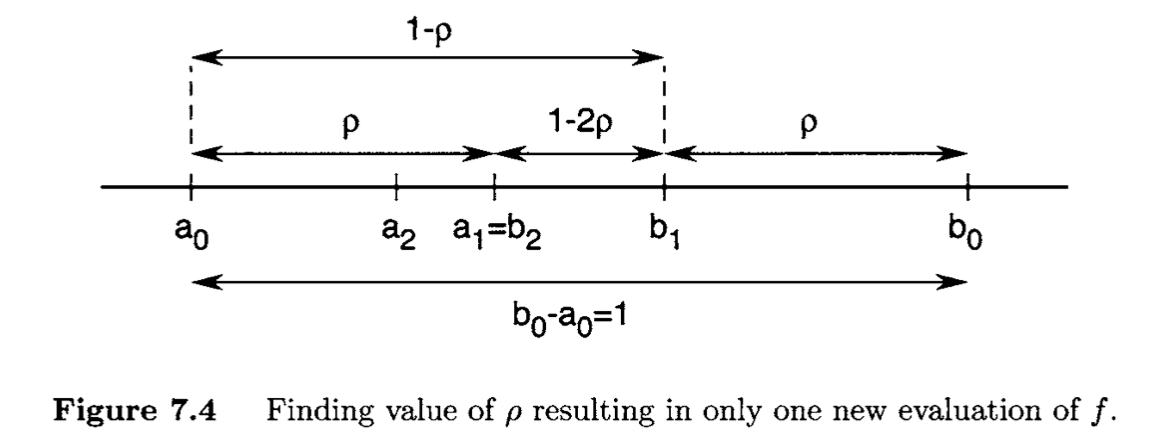
We then evaluate $f$ at the intermediate points. If $f(a_1)<f(b_1)$, then the minimizer must lie in the range $[a_0, b_1]$. If, on the other hand, $f(a_1) \ge f(b_1)$, then the minimizer is located in the range $[a_1, b_0]$.

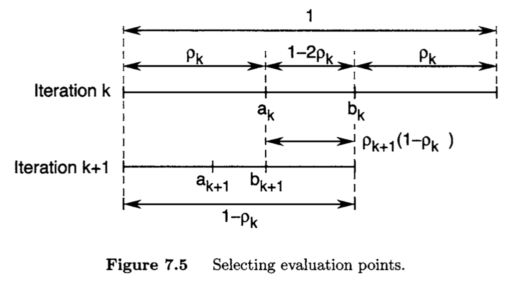
Suppose, for example, that $f(a_1)<f(b_q)$. Then, we know that $x^* \in [a_0,b_1]$. Because $a_1$ is already in the uncertainty interval and $f(a_1)$ is already known, we can make $a_1$ coincide with $b_2$. Thus, only one new evaluation of $f$ at $a_2$ would be necessary. To find the value of $p$ that results in only one new evaluation of $f$, see Figure 7.4. Without loss of generality, imagine that the original range $[a_0, b_0]$ is of unit length. Then, to have only one new evaluation of $f$ it is enough to choose $\rho$ so that

$$\begin{gather*} \rho(b_1-a_0)=b_1-b_2. \end{gather*}$$

Because $b_1-a_0=1-\rho$ and $b_1-b_2=1-2\rho$, we have

$$\begin{gather*} \rho(1-\rho)=1-2\rho. \end{gather*}$$

We write the quadratic equation above as

$$\begin{gather*} \rho^2-3\rho+1=0. \end{gather*}$$

The solutions are

$$\begin{gather*} \rho_1={3+\sqrt{5} \over 2},\;\;\rho_2={3-\sqrt{5} \over 2}. \end{gather*}$$

Because we require that $\rho<{1\over 2}$, we take

$$\begin{gather*} \rho={3-\sqrt{5} \over 2} \approx 0.382. \end{gather*}$$

Observe that

$$\begin{gather*} {\rho \over 1-\rho} = {3-\sqrt{5}\over \sqrt{5}-1}={\sqrt{5}-1\over 2}={1-\rho\over 1}, \end{gather*}$$

that is,

$$\begin{gather*} {\rho\over 1-\rho}={1-\rho\over 1}. \end{gather*}$$

Using this method, the uncertainty range is reduced by the ratio $1-\rho \approx 0.61803$ at every stage. Hence, $N$ steps of reduction using the golden section method reduces the range by the factor

$$\begin{gather*} (1-\rho)^N\approx (0.61803)^N. \end{gather*}$$

Fobonacci Method

Instead of using the same $\rho$, we are allowed to vary the valye $\rho$ from stage to stage, so that at the $k$th stage in the reduction process we use a value $\rho_k$, at the next stage we use a value $\rho_{k+1}$, and so on.

To derive the strategy for selecting evaluation points, consider Figure 7.5. We see that it is sufficient to choose the $\rho_k$ such that

$$\begin{gather*} \rho_{k+1}(1-\rho_k)=1-2\rho_k. \end{gather*}$$

After some manipulations, we obtain

$$\begin{gather*} \rho_{k+1}=1-{\rho_k\over 1-\rho_k}. \end{gather*}$$

Suppose that we are given a sequence $\rho_1, \rho_2,\cdots$ satisfying the conditions above and we use this sequence in our search algorithm. Then, after $N$ iterations of the algorithm, the uncertainty range is reduced by a factor of

$$\begin{gather*} (1-\rho_1)(1-\rho_2)\cdots(1-\rho_N) \end{gather*}$$

We therefore want to

$$\begin{align*} \text{minimize}\;\; & (1-\rho_1)(1-\rho_2)\cdots(1-\rho_N) \\ \text{subject to}\;\; & \rho_{k+1}=1-{\rho_k\over 1-\rho_k},k=1,\cdots,N-1 \\ & 0\le\rho_k\le{1\over 2},k=1,\cdots,N. \end{align*}$$

Fibonacci Sequence

The sequence is defined as follows. First, let $F_{-1}=0$ and $F_0=1$ by convention. Then, for $k \ge 0$,

$$\begin{gather*} F_{k+1}=F_k+F_{k-1}. \end{gather*}$$

It turns out that the solution to the optimization problem above is

$$\begin{align*} \rho_1 & = 1-{F_N\over F_{N+1}}, \\ \rho_2 & = 1-{F_{N-1}\over F_{N}}, \\ & \vdots \\ \rho_k & = 1-{F_{N-k+1}\over F_{N-k+2}}, \\ & \vdots \\ \rho_N & = 1-{F_1\over F_2}, \end{align*}$$

where the $F_k$ are the elements of the Fibonacci sequence. The resulting algorithm is called the Fibonacci search method.
The uncertainty range is reduced by the factor

$$\begin{gather*} (1-\rho_1)(1-\rho_2)\cdots(1-\rho_N) = {F_N\over F_{N+1}}{F_{N-1}\over F_N}\cdots {F_1\over F_2}={F_1\over F_{N+1}}={1\over F_{N+1}}. \end{gather*}$$

The Fibonnaci method is better than the golden section method in that it gives a smaller final uncertainty range.
We point out that there is an anomaly in the final iteration of the Fibonacci search method, because

$$\begin{gather*} \rho_N=1-{F_1\over F_2}={1\over 2}. \end{gather*}$$

To get arounf this problem, we perform the new evaluation for the last iteration using $\rho_N=1/2-\varepsilon$, where $\varepsilon$ is a small number. Therefore,

$$\begin{gather*} 1-\rho_N={1\over 2} \\ 1-(\rho_N-\varepsilon)={1\over2}+\varepsilon={1+2\varepsilon\over2}, \end{gather*}$$

Therefore, in the worst case, the reduction factor in the uncertainty range for the Fibonacci method is

$$\begin{gather*} {1+2\varepsilon\over F_{N+1}}. \end{gather*}$$

Lemma 1

For $k\ge 2$,

$$\begin{gather*} r_k=-{F_{k-2}-F_{k-1}r_1\over F_{k-3}-F_{k-2}r_1}. \end{gather*}$$

Proof of Lemma 1

We proceed by induction. For $k=2$ we have

$$\begin{gather*} r_2={1\over r_1}-1={1-r_1\over r_1}=-{F_0-F_1r_1\over F_{-1}-F_0r_1} \end{gather*}$$

and hence the lemma holds for k=2, Suppose now that the lemma holds for $k\ge 2$. We show that it also holds for $k+1$. We have

$$\begin{align*} r_{k+1} & = {1\over r_k}-1 \\ & = {F_{k-3}+F_{k-2}r_1\over F_{k-2}-F_{k-1}r_1}-{F_{k-2}-F_{k-1}r_1\over F_{k-2}-F_{k-1}r_1} \\ & = -{F_{k-2}+F_{k-3}-(F_{k-1}+F_{k-2})r_1\over F_{k-2}-F_{k-1}r_1} \\ & = -{F_{k-1}-F_kr_1\over F_{k-2}-F_{k-1}r_1}, \end{align*}$$

where we used the formation law for the Fibonacci sequence.

Lemma 2

For $k\ge 2$,

$$\begin{gather*} (-1)^k(F_{k-2}-F_{k-1}r_1)>0. \end{gather*}$$

Proof of Lemma 2

We proceed by induction. For $k=2$, we have

$$\begin{gather*} (-1)^2(F_0-F_1r_1)=1-r_1. \end{gather*}$$

But $r_1=1/(1+r_2) \le 2/3$, and hence $1-r_1>0$. Therefore, the result holds for $k=2$. Suppose now that the lemma holds for $k\ge 2$. We show that it also holds for $k+1$. We have

$$\begin{gather*} (-1)^{k+1}(F_{k-1}-F_kr_1)=(-1)^{k+1}r_{k+1}{1\over r_{k+1}}(F_{k-1}-F_kr_1). \end{gather*}$$

By Lemma 1,

$$\begin{gather*} r_{k+1}=-{F_{k-1}-F_kr_1 \over F_{k-2}-F_{k-1}r_1}. \end{gather*}$$

Substituting for $1/r_{k+1}$, we obtain

$$\begin{gather*} (-1)^{k+1}(F_{k-1}-F_kr_1)=r_{k+1}(-1)^k(F_{k-2}-F_{k-1}r_1)>0, \end{gather*}$$

which completes the proof.

Lemma 3

For $k \ge 2$,

$$\begin{gather*} (-1)^{k+1}r_1\ge (-1)^{k+1}{F_k\over F_{k+1}}. \end{gather*}$$

Proof of Lemma 3

Because $r_{k+1}={1\over r_k}-1$ and $r_k \ge {1\over2}$, we have $r_{k+1}\ge 1$. Substituting for $r_{k+1}$ from Lemma 1, we get

$$\begin{gather*} -{F_{k-1}-F_kr_1\over F_{k-2}-F_{k-1}r_1}\le 1. \end{gather*}$$

Multiplying the numerator and denominator by $(-1)^k$ yields

$$\begin{gather*} {(-1)^{k+1}(F_{k-1}-F_kr_1)\over (-1)^k(F_{k-2}-F_{k-1}r_1)}\le 1. \end{gather*}$$

By Lemma 2, $(-1)^k(F_{k-2}-F_{k-1}r_1)>0$, and therefore we can multiply both sides of the inequality above by $(-1)^k(F{k-2}-F{k-1}r_1) to obtain

$$\begin{gather*} (-1)^{k+1}(F_{k-1}-F_kr_1) \le (-1)^k(F_{k-2}-F_{k-1}r_1). \end{gather*}$$

Rearranging yields

$$\begin{gather*} (-1)^{k+1}(F_{k-1}+F_k)r_1 \ge (-1)^{k+1}(F_{k-2}+F_{k-1}). \end{gather*}$$

Using the law of formation of the Fibonacci sequence, we get

$$\begin{gather*} (-1)^{k+1}F_{k+1}r_1 \ge (-1)^{k+1}F_k, \end{gather*}$$

which upon dividing by $F_{k+1}$ on both sides gives the desired result.

Theorem (Optimality of the Fibonacci Method)

Let $r_1,\cdots,r_N,N\ge 2$, satisfy the constraints

$$\begin{gather*} r_{k+1}={1\over r_k}-1, k=1,\cdots,N-1, \\ r_k \ge {1\over 2}, k=1,\cdots,N. \end{gather*}$$

Then,

$$\begin{gather*} r_1\cdots r_N \ge {1\over F_{N+1}}. \end{gather*}$$

Furthermore,

$$\begin{gather*} r_1\cdots r_N = {1\over F_{N+1}} \end{gather*}$$

if and only if $r_k=F_{N-k+1}/F_{N-k+2}, k=1,\cdots,N$. In other words, the values of $r_1,\cdots,r_N$ used in the Fibonacci search method form a unique solution to the optimization problem.

Proof

By substituting expressions for $r_1,\cdots,r_N$ from Lemma 1 and performing the appropriate cancellations, we obtain

$$\begin{gather*} r_1\cdots r_N=(-1)^N(F_{N-2}-F_{N-1}r_1)=(-1)^NF_{N-2}+F_{N-1}(-1)^{N+1}r_1. \end{gather*}$$

Using Lemma 3 yields

$$\begin{align*} r_1\cdots r_N & \ge (-1)^NF_{N-2}+F_{N-1}(-1)^{N+1}{F_N\over F_{N+1}} \\ & = (-1)^N(F_{N-2}F_{N+1}-F_{N-1}F_N){1\over F_{N+1}}. \end{align*}$$

The following holds: $(-1)^N(F_{N-2}F_{N+1}-F_{N-1}F_N)=1$ (You can trust me here, easy to prove on you own using induction). Hence,

$$\begin{gather*} r_1\cdots r_N\ge {1\over F_{N+1}}. \end{gather*}$$

From the above we see that

$$\begin{gather*} r_1\cdots r_N = {1\over F_{N+1}}. \end{gather*}$$

if and only if

$$\begin{gather*} r_1 = {F_N\over F_{N+1}}. \end{gather*}$$

This is simply the value of $r_1$ for the Fibonacci search method.

Bisection Method

The bisection method is a simple algorithm for successively reducing the uncertainty interval based on evaluations of the derivative. To begin, let $x^{(0)}=(a_0+b_0)/2$ be the midpoint of the initial uncertainty interval. Next, evaluate $f'(x^(0))$. If $f'(x^{(0)})>0$, then we deduce that the minimizer lies to the left of $x^{(0)}$. On the other hand, if $f'(x^{(0)})<0$, then we deduce that the minimizer lies to the right of $x^{(0)}$. Finally, if $f'(x^{(0)})=0$, then we declare $x^{(0)}$ to be the minimizer and terminate our search.
The uncertainty interval is reduced by a factor of $(1/2)^N$.

Newton's Method

We assume now that at each measurement point $x^{(k)}$ we can determine $f(x^{(k)}),f'(x^{(k)}),f''(x^{(k)})$. We can fit a quadratic function through $x^{(k)}$ that matches its first and second derivatives with that of the function f. This quadratic has the form

$$\begin{gather*} q(x)=f(x^{(k)})+f'(x^{(k)})(x-x^{(k)})+{1\over 2}f''(x^{(k)})(x-x^{(k)})^2. \end{gather*}$$

Then, instead of minimizing $f$, we minimize its approximation $q$. The first-order neccesary condition for a minimizer of $q$ yields

$$\begin{gather*} 0=q'(x)=f'(x^{(k)})+f''(x^{(k)})(x-x^{(k)}). \end{gather*}$$

Setting $x=x^{(k+1)}$, we obtain

$$\begin{gather*} x^{(k+1)} = x^{(k)} - {f'(x^{(k)}) \over f''(x^{(k)})}. \end{gather*}$$